Raise your ELBO
Published on 2019-02-14
Table of Contents
In this post I give an introduction to variational inference, which is about maximising the evidence lower bound (ELBO).
I use a top-down approach, starting with the KL divergence and the ELBO, to lay the mathematical framework of all the models in this post.
Then I define mixture models and the EM algorithm, with Gaussian mixture model (GMM), probabilistic latent semantic analysis (pLSA) and the hidden markov model (HMM) as examples.
After that I present the fully Bayesian version of EM, also known as mean field approximation (MFA), and apply it to fully Bayesian mixture models, with fully Bayesian GMM (also known as variational GMM), latent Dirichlet allocation (LDA) and Dirichlet process mixture model (DPMM) as examples.
Then I explain stochastic variational inference, a modification of EM and MFA to improve efficiency.
Finally I talk about autoencoding variational Bayes (AEVB), a Monte-Carlo + neural network approach to raising the ELBO, exemplified by the variational autoencoder (VAE). I also show its fully Bayesian version.
Acknowledgement. The following texts and resources were illuminating during the writing of this post: the Stanford CS228 notes (1,2), the Tel Aviv Algorithms in Molecular Biology slides (clear explanations of the connection between EM and Baum-Welch), Chapter 10 of Bishop's book (brilliant introduction to variational GMM), Section 2.5 of Sudderth's thesis and metacademy. Also thanks to Josef Lindman Hörnlund for discussions. The research was done while working at KTH mathematics department.
If you are reading on a mobile device, you may need to "request desktop site" for the equations to be properly displayed. This post is licensed under CC BY-SA and GNU FDL.
KL divergence and ELBO
Let \(p\) and \(q\) be two probability measures. The Kullback-Leibler (KL) divergence is defined as
\[D(q||p) = E_q \log{q \over p}.\]
It achieves minimum \(0\) when \(p = q\).
If \(p\) can be further written as
\[p(x) = {w(x) \over Z}, \qquad (0)\]
where \(Z\) is a normaliser, then
\[\log Z = D(q||p) + L(w, q), \qquad(1)\]
where \(L(w, q)\) is called the evidence lower bound (ELBO), defined by
\[L(w, q) = E_q \log{w \over q}. \qquad (1.25)\]
From (1), we see that to minimise the nonnegative term \(D(q || p)\), one can maximise the ELBO.
To this end, we can simply discard \(D(q || p)\) in (1) and obtain:
\[\log Z \ge L(w, q) \qquad (1.3)\]
and keep in mind that the inequality becomes an equality when \(q = {w \over Z}\).
It is time to define the task of variational inference (VI), also known as variational Bayes (VB).
Definition. Variational inference is concerned with maximising the ELBO \(L(w, q)\).
There are mainly two versions of VI, the half Bayesian and the fully Bayesian cases. Half Bayesian VI, to which expectation-maximisation algorithms (EM) apply, instantiates (1.3) with
\[\begin{aligned} Z &= p(x; \theta)\\ w &= p(x, z; \theta)\\ q &= q(z) \end{aligned}\]
and the dummy variable \(x\) in Equation (0) is substituted with \(z\).
Fully Bayesian VI, often just called VI, has the following instantiations:
\[\begin{aligned} Z &= p(x) \\ w &= p(x, z, \theta) \\ q &= q(z, \theta) \end{aligned}\]
and \(x\) in Equation (0) is substituted with \((z, \theta)\).
In both cases \(\theta\) are parameters and \(z\) are latent variables.
Remark on the naming of things. The term "variational" comes from the fact that we perform calculus of variations: maximise some functional (\(L(w, q)\)) over a set of functions (\(q\)). Note however, most of the VI / VB algorithms do not concern any techniques in calculus of variations, but only uses Jensen's inequality / the fact the \(D(q||p)\) reaches minimum when \(p = q\). Due to this reasoning of the naming, EM is also a kind of VI, even though in the literature VI often referes to its fully Bayesian version.
EM
To illustrate the EM algorithms, we first define the mixture model.
Definition (mixture model). Given dataset \(x_{1 : m}\), we assume the data has some underlying latent variable \(z_{1 : m}\) that may take a value from a finite set \(\{1, 2, ..., n_z\}\). Let \(p(z_{i}; \pi)\) be categorically distributed according to the probability vector \(\pi\). That is, \(p(z_{i} = k; \pi) = \pi_k\). Also assume \(p(x_{i} | z_{i} = k; \eta) = p(x_{i}; \eta_k)\). Find \(\theta = (\pi, \eta)\) that maximises the likelihood \(p(x_{1 : m}; \theta)\).
Represented as a DAG (a.k.a the plate notations), the model looks like this:
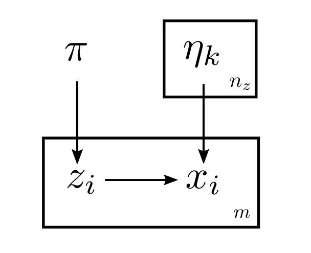
where the boxes with \(m\) mean repitition for \(m\) times, since there \(m\) indepdent pairs of \((x, z)\), and the same goes for \(\eta\).
The direct maximisation
\[\max_\theta \sum_i \log p(x_{i}; \theta) = \max_\theta \sum_i \log \int p(x_{i} | z_i; \theta) p(z_i; \theta) dz_i\]
is hard because of the integral in the log.
We can fit this problem in (1.3) by having \(Z = p(x_{1 : m}; \theta)\) and \(w = p(z_{1 : m}, x_{1 : m}; \theta)\). The plan is to update \(\theta\) repeatedly so that \(L(p(z, x; \theta_t), q(z))\) is non decreasing over time \(t\).
Equation (1.3) at time \(t\) for the $i$th datapoint is
\[\log p(x_{i}; \theta_t) \ge L(p(z_i, x_{i}; \theta_t), q(z_i)) \qquad (2)\]
Each timestep consists of two steps, the E-step and the M-step.
At E-step, we set
\[q(z_{i}) = p(z_{i}|x_{i}; \theta_t), \]
to turn the inequality into equality. We denote \(r_{ik} = q(z_i = k)\) and call them responsibilities, so the posterior \(q(z_i)\) is categorical distribution with parameter \(r_i = r_{i, 1 : n_z}\).
At M-step, we maximise \(\sum_i L(p(x_{i}, z_{i}; \theta), q(z_{i}))\) over \(\theta\):
\[\begin{aligned} \theta_{t + 1} &= \text{argmax}_\theta \sum_i L(p(x_{i}, z_{i}; \theta), p(z_{i} | x_{i}; \theta_t)) \\ &= \text{argmax}_\theta \sum_i \mathbb E_{p(z_{i} | x_{i}; \theta_t)} \log p(x_{i}, z_{i}; \theta) \qquad (2.3) \end{aligned}\]
So \(\sum_i L(p(x_{i}, z_{i}; \theta), q(z_i))\) is non-decreasing at both the E-step and the M-step.
We can see from this derivation that EM is half-Bayesian. The E-step is Bayesian it computes the posterior of the latent variables and the M-step is frequentist because it performs maximum likelihood estimate of \(\theta\).
It is clear that the ELBO sum coverges as it is nondecreasing with an upper bound, but it is not clear whether the sum converges to the correct value, i.e. \(\max_\theta p(x_{1 : m}; \theta)\). In fact it is said that the EM does get stuck in local maximum sometimes.
A different way of describing EM, which will be useful in hidden Markov model is:
- At E-step, one writes down the formula \[\sum_i \mathbb E_{p(z_i | x_{i}; \theta_t)} \log p(x_{i}, z_i; \theta). \qquad (2.5)\]
- At M-setp, one finds \(\theta_{t + 1}\) to be the \(\theta\) that maximises the above formula.
GMM
Gaussian mixture model (GMM) is an example of mixture models.
The space of the data is \(\mathbb R^n\). We use the hypothesis that the data is Gaussian conditioned on the latent variable:
\[(x_i; \eta_k) \sim N(\mu_k, \Sigma_k),\]
so we write \(\eta_k = (\mu_k, \Sigma_k)\),
During E-step, the \(q(z_i)\) can be directly computed using Bayes' theorem:
\[r_{ik} = q(z_i = k) = \mathbb P(z_i = k | x_{i}; \theta_t) = {g_{\mu_{t, k}, \Sigma_{t, k}} (x_{i}) \pi_{t, k} \over \sum_{j = 1 : n_z} g_{\mu_{t, j}, \Sigma_{t, j}} (x_{i}) \pi_{t, j}},\]
where \(g_{\mu, \Sigma} (x) = (2 \pi)^{- n / 2} \det \Sigma^{-1 / 2} \exp(- {1 \over 2} (x - \mu)^T \Sigma^{-1} (x - \mu))\) is the pdf of the Gaussian distribution \(N(\mu, \Sigma)\).
During M-step, we need to compute
\[\text{argmax}_{\Sigma, \mu, \pi} \sum_{i = 1 : m} \sum_{k = 1 : n_z} r_{ik} \log (g_{\mu_k, \Sigma_k}(x_{i}) \pi_k).\]
This is similar to the quadratic discriminant analysis, and the solution is
\[\begin{aligned} \pi_{k} &= {1 \over m} \sum_{i = 1 : m} r_{ik}, \\ \mu_{k} &= {\sum_i r_{ik} x_{i} \over \sum_i r_{ik}}, \\ \Sigma_{k} &= {\sum_i r_{ik} (x_{i} - \mu_{t, k}) (x_{i} - \mu_{t, k})^T \over \sum_i r_{ik}}. \end{aligned}\]
Remark. The k-means algorithm is the \(\epsilon \to 0\) limit of the GMM with constraints \(\Sigma_k = \epsilon I\). See Section 9.3.2 of Bishop 2006 for derivation. It is also briefly mentioned there that a variant in this setting where the covariance matrix is not restricted to \(\epsilon I\) is called elliptical k-means algorithm.
SMM
As a transition to the next models to study, let us consider a simpler mixture model obtained by making one modification to GMM: change \((x; \eta_k) \sim N(\mu_k, \Sigma_k)\) to \(\mathbb P(x = w; \eta_k) = \eta_{kw}\) where \(\eta\) is a stochastic matrix and \(w\) is an arbitrary element of the space for \(x\). So now the space for both \(x\) and \(z\) are finite. We call this model the simple mixture model (SMM).
As in GMM, at E-step \(r_{ik}\) can be explicitly computed using Bayes' theorem.
It is not hard to write down the solution to the M-step in this case:
\[\begin{aligned} \pi_{k} &= {1 \over m} \sum_i r_{ik}, \qquad (2.7)\\ \eta_{k, w} &= {\sum_i r_{ik} 1_{x_i = w} \over \sum_i r_{ik}}. \qquad (2.8) \end{aligned}\]
where \(1_{x_i = w}\) is the indicator function, and evaluates to \(1\) if \(x_i = w\) and \(0\) otherwise.
Two trivial variants of the SMM are the two versions of probabilistic latent semantic analysis (pLSA), which we call pLSA1 and pLSA2.
The model pLSA1 is a probabilistic version of latent semantic analysis, which is basically a simple matrix factorisation model in collaborative filtering, whereas pLSA2 has a fully Bayesian version called latent Dirichlet allocation (LDA), not to be confused with the other LDA (linear discriminant analysis).
pLSA
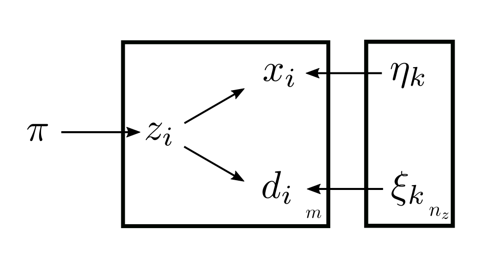
The pLSA model (Hoffman 2000) is a mixture model, where the dataset is now pairs \((d_i, x_i)_{i = 1 : m}\). In natural language processing, \(x\) are words and \(d\) are documents, and a pair \((d, x)\) represent an ocurrance of word \(x\) in document \(d\).
For each datapoint \((d_{i}, x_{i})\),
\[\begin{aligned} p(d_i, x_i; \theta) &= \sum_{z_i} p(z_i; \theta) p(d_i | z_i; \theta) p(x_i | z_i; \theta) \qquad (2.91)\\ &= p(d_i; \theta) \sum_z p(x_i | z_i; \theta) p (z_i | d_i; \theta) \qquad (2.92). \end{aligned}\]
Of the two formulations, (2.91) corresponds to pLSA type 1, and (2.92) corresponds to type 2.
pLSA1
The pLSA1 model (Hoffman 2000) is basically SMM with \(x_i\) substituted with \((d_i, x_i)\), which conditioned on \(z_i\) are independently categorically distributed:
\[p(d_i = u, x_i = w | z_i = k; \theta) = p(d_i ; \xi_k) p(x_i; \eta_k) = \xi_{ku} \eta_{kw}.\]
The model can be illustrated in the plate notations:
So the solution of the M-step is
\[\begin{aligned} \pi_{k} &= {1 \over m} \sum_i r_{ik} \\ \xi_{k, u} &= {\sum_i r_{ik} 1_{d_{i} = u} \over \sum_i r_{ik}} \\ \eta_{k, w} &= {\sum_i r_{ik} 1_{x_{i} = w} \over \sum_i r_{ik}}. \end{aligned}\]
Remark. pLSA1 is the probabilistic version of LSA, also known as matrix factorisation.
Let \(n_d\) and \(n_x\) be the number of values \(d_i\) and \(x_i\) can take.
Problem (LSA). Let \(R\) be a \(n_d \times n_x\) matrix, fix \(s \le \min\{n_d, n_x\}\). Find \(n_d \times s\) matrix \(D\) and \(n_x \times s\) matrix \(X\) that minimises
\[J(D, X) = \|R - D X^T\|_F.\]
where \(\|\cdot\|_F\) is the Frobenius norm.
Claim. Let \(R = U \Sigma V^T\) be the SVD of \(R\), then the solution to the above problem is \(D = U_s \Sigma_s^{{1 \over 2}}\) and \(X = V_s \Sigma_s^{{1 \over 2}}\), where \(U_s\) (resp. \(V_s\)) is the matrix of the first \(s\) columns of \(U\) (resp. \(V\)) and \(\Sigma_s\) is the \(s \times s\) submatrix of \(\Sigma\).
One can compare pLSA1 with LSA. Both procedures produce embeddings of \(d\) and \(x\): in pLSA we obtain \(n_z\) dimensional embeddings \(\xi_{\cdot, u}\) and \(\eta_{\cdot, w}\), whereas in LSA we obtain \(s\) dimensional embeddings \(D_{u, \cdot}\) and \(X_{w, \cdot}\).
pLSA2
Let us turn to pLSA2 (Hoffman 2004), corresponding to (2.92). We rewrite it as
\[p(x_i | d_i; \theta) = \sum_{z_i} p(x_i | z_i; \theta) p(z_i | d_i; \theta).\]
To simplify notations, we collect all the $xi$s with the corresponding \(d_i\) equal to 1 (suppose there are \(m_1\) of them), and write them as \((x_{1, j})_{j = 1 : m_1}\). In the same fashion we construct \(x_{2, 1 : m_2}, x_{3, 1 : m_3}, ... x_{n_d, 1 : m_{n_d}}\). Similarly, we relabel the corresponding \(d_i\) and \(z_i\) accordingly.
With almost no loss of generality, we assume all $mℓ$s are equal and write them as \(m\).
Now the model becomes
\[p(x_{\ell, i} | d_{\ell, i} = \ell; \theta) = \sum_k p(x_{\ell, i} | z_{\ell, i} = k; \theta) p(z_{\ell, i} = k | d_{\ell, i} = \ell; \theta).\]
Since we have regrouped the \(x\)'s and \(z\)'s whose indices record the values of the \(d\)'s, we can remove the \(d\)'s from the equation altogether:
\[p(x_{\ell, i}; \theta) = \sum_k p(x_{\ell, i} | z_{\ell, i} = k; \theta) p(z_{\ell, i} = k; \theta).\]
It is effectively a modification of SMM by making \(n_d\) copies of \(\pi\). More specifically the parameters are \(\theta = (\pi_{1 : n_d, 1 : n_z}, \eta_{1 : n_z, 1 : n_x})\), where we model \((z | d = \ell) \sim \text{Cat}(\pi_{\ell, \cdot})\) and, as in pLSA1, \((x | z = k) \sim \text{Cat}(\eta_{k, \cdot})\).
Illustrated in the plate notations, pLSA2 is:
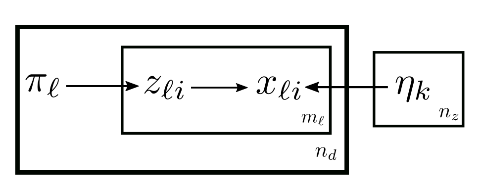
The computation is basically adding an index \(\ell\) to the computation of SMM wherever applicable.
The updates at the E-step is
\[r_{\ell i k} = p(z_{\ell i} = k | x_{\ell i}; \theta) \propto \pi_{\ell k} \eta_{k, x_{\ell i}}.\]
And at the M-step
\[\begin{aligned} \pi_{\ell k} &= {1 \over m} \sum_i r_{\ell i k} \\ \eta_{k w} &= {\sum_{\ell, i} r_{\ell i k} 1_{x_{\ell i} = w} \over \sum_{\ell, i} r_{\ell i k}}. \end{aligned}\]
HMM
The hidden markov model (HMM) is a sequential version of SMM, in the same sense that recurrent neural networks are sequential versions of feed-forward neural networks.
HMM is an example where the posterior \(p(z_i | x_i; \theta)\) is not easy to compute, and one has to utilise properties of the underlying Bayesian network to go around it.
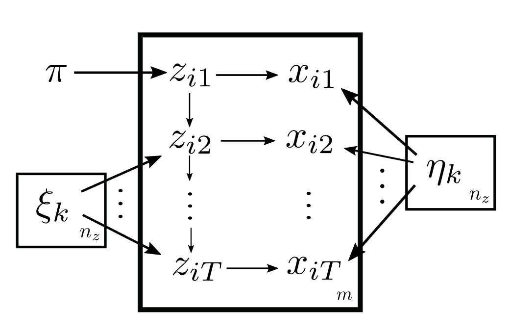
Now each sample is a sequence \(x_i = (x_{ij})_{j = 1 : T}\), and so are the latent variables \(z_i = (z_{ij})_{j = 1 : T}\).
The latent variables are assumed to form a Markov chain with transition matrix \((\xi_{k \ell})_{k \ell}\), and \(x_{ij}\) is completely dependent on \(z_{ij}\):
\[\begin{aligned} p(z_{ij} | z_{i, j - 1}) &= \xi_{z_{i, j - 1}, z_{ij}},\\ p(x_{ij} | z_{ij}) &= \eta_{z_{ij}, x_{ij}}. \end{aligned}\]
Also, the distribution of \(z_{i1}\) is again categorical with parameter \(\pi\):
\[p(z_{i1}) = \pi_{z_{i1}}\]
So the parameters are \(\theta = (\pi, \xi, \eta)\). And HMM can be shown in plate notations as:
Now we apply EM to HMM, which is called the Baum-Welch algorithm. Unlike the previous examples, it is too messy to compute \(p(z_i | x_{i}; \theta)\), so during the E-step we instead write down formula (2.5) directly in hope of simplifying it:
\[\begin{aligned} \mathbb E_{p(z_i | x_i; \theta_t)} \log p(x_i, z_i; \theta_t) &=\mathbb E_{p(z_i | x_i; \theta_t)} \left(\log \pi_{z_{i1}} + \sum_{j = 2 : T} \log \xi_{z_{i, j - 1}, z_{ij}} + \sum_{j = 1 : T} \log \eta_{z_{ij}, x_{ij}}\right). \qquad (3) \end{aligned}\]
Let us compute the summand in second term:
\[\begin{aligned} \mathbb E_{p(z_i | x_{i}; \theta_t)} \log \xi_{z_{i, j - 1}, z_{ij}} &= \sum_{k, \ell} (\log \xi_{k, \ell}) \mathbb E_{p(z_{i} | x_{i}; \theta_t)} 1_{z_{i, j - 1} = k, z_{i, j} = \ell} \\ &= \sum_{k, \ell} p(z_{i, j - 1} = k, z_{ij} = \ell | x_{i}; \theta_t) \log \xi_{k, \ell}. \qquad (4) \end{aligned}\]
Similarly, one can write down the first term and the summand in the third term to obtain
\[\begin{aligned} \mathbb E_{p(z_i | x_{i}; \theta_t)} \log \pi_{z_{i1}} &= \sum_k p(z_{i1} = k | x_{i}; \theta_t), \qquad (5) \\ \mathbb E_{p(z_i | x_{i}; \theta_t)} \log \eta_{z_{i, j}, x_{i, j}} &= \sum_{k, w} 1_{x_{ij} = w} p(z_{i, j} = k | x_i; \theta_t) \log \eta_{k, w}. \qquad (6) \end{aligned}\]
plugging (4)(5)(6) back into (3) and summing over \(j\), we obtain the formula to maximise over \(\theta\) on:
\[\sum_k \sum_i r_{i1k} \log \pi_k + \sum_{k, \ell} \sum_{j = 2 : T, i} s_{ijk\ell} \log \xi_{k, \ell} + \sum_{k, w} \sum_{j = 1 : T, i} r_{ijk} 1_{x_{ij} = w} \log \eta_{k, w},\]
where
\[\begin{aligned} r_{ijk} &:= p(z_{ij} = k | x_{i}; \theta_t), \\ s_{ijk\ell} &:= p(z_{i, j - 1} = k, z_{ij} = \ell | x_{i}; \theta_t). \end{aligned}\]
Now we proceed to the M-step. Since each of the \(\pi_k, \xi_{k, \ell}, \eta_{k, w}\) is nicely confined in the inner sum of each term, together with the constraint \(\sum_k \pi_k = \sum_\ell \xi_{k, \ell} = \sum_w \eta_{k, w} = 1\) it is not hard to find the argmax at time \(t + 1\) (the same way one finds the MLE for any categorical distribution):
\[\begin{aligned} \pi_{k} &= {1 \over m} \sum_i r_{i1k}, \qquad (6.1) \\ \xi_{k, \ell} &= {\sum_{j = 2 : T, i} s_{ijk\ell} \over \sum_{j = 1 : T - 1, i} r_{ijk}}, \qquad(6.2) \\ \eta_{k, w} &= {\sum_{ij} 1_{x_{ij} = w} r_{ijk} \over \sum_{ij} r_{ijk}}. \qquad(6.3) \end{aligned}\]
Note that (6.1)(6.3) are almost identical to (2.7)(2.8). This makes sense as the only modification HMM makes over SMM is the added dependencies between the latent variables.
What remains is to compute \(r\) and \(s\).
This is done by using the forward and backward procedures which takes advantage of the conditioned independence / topology of the underlying Bayesian network. It is out of scope of this post, but for the sake of completeness I include it here.
Let
\[\begin{aligned} \alpha_k(i, j) &:= p(x_{i, 1 : j}, z_{ij} = k; \theta_t), \\ \beta_k(i, j) &:= p(x_{i, j + 1 : T} | z_{ij} = k; \theta_t). \end{aligned}\]
They can be computed recursively as
\[\begin{aligned} \alpha_k(i, j) &= \begin{cases} \eta_{k, x_{1j}} \pi_k, & j = 1; \\ \eta_{k, x_{ij}} \sum_\ell \alpha_\ell(j - 1, i) \xi_{k\ell}, & j \ge 2. \end{cases}\\ \beta_k(i, j) &= \begin{cases} 1, & j = T;\\ \sum_\ell \xi_{k\ell} \beta_\ell(j + 1, i) \eta_{\ell, x_{i, j + 1}}, & j < T. \end{cases} \end{aligned}\]
Then
\[\begin{aligned} p(z_{ij} = k, x_{i}; \theta_t) &= \alpha_k(i, j) \beta_k(i, j), \qquad (7)\\ p(x_{i}; \theta_t) &= \sum_k \alpha_k(i, j) \beta_k(i, j),\forall j = 1 : T \qquad (8)\\ p(z_{i, j - 1} = k, z_{i, j} = \ell, x_{i}; \theta_t) &= \alpha_k(i, j) \xi_{k\ell} \beta_\ell(i, j + 1) \eta_{\ell, x_{j + 1, i}}. \qquad (9) \end{aligned}\]
And this yields \(r_{ijk}\) and \(s_{ijk\ell}\) since they can be computed as \({(7) \over (8)}\) and \({(9) \over (8)}\) respectively.
Fully Bayesian EM / MFA
Let us now venture into the realm of full Bayesian.
In EM we aim to maximise the ELBO
\[\int q(z) \log {p(x, z; \theta) \over q(z)} dz d\theta\]
alternately over \(q\) and \(\theta\). As mentioned before, the E-step of maximising over \(q\) is Bayesian, in that it computes the posterior of \(z\), whereas the M-step of maximising over \(\theta\) is maximum likelihood and frequentist.
The fully Bayesian EM makes the M-step Bayesian by making \(\theta\) a random variable, so the ELBO becomes
\[L(p(x, z, \theta), q(z, \theta)) = \int q(z, \theta) \log {p(x, z, \theta) \over q(z, \theta)} dz d\theta\]
We further assume \(q\) can be factorised into distributions on \(z\) and \(\theta\): \(q(z, \theta) = q_1(z) q_2(\theta)\). So the above formula is rewritten as
\[L(p(x, z, \theta), q(z, \theta)) = \int q_1(z) q_2(\theta) \log {p(x, z, \theta) \over q_1(z) q_2(\theta)} dz d\theta\]
To find argmax over \(q_1\), we rewrite
\[\begin{aligned} L(p(x, z, \theta), q(z, \theta)) &= \int q_1(z) \left(\int q_2(\theta) \log p(x, z, \theta) d\theta\right) dz - \int q_1(z) \log q_1(z) dz - \int q_2(\theta) \log q_2(\theta) \\&= - D(q_1(z) || p_x(z)) + C, \end{aligned}\]
where \(p_x\) is a density in \(z\) with
\[\log p_x(z) = \mathbb E_{q_2(\theta)} \log p(x, z, \theta) + C.\]
So the \(q_1\) that maximises the ELBO is \(q_1^* = p_x\).
Similarly, the optimal \(q_2\) is such that
\[\log q_2^*(\theta) = \mathbb E_{q_1(z)} \log p(x, z, \theta) + C.\]
The fully Bayesian EM thus alternately evaluates \(q_1^*\) (E-step) and \(q_2^*\) (M-step).
It is also called mean field approximation (MFA), and can be easily generalised to models with more than two groups of latent variables, see e.g. Section 10.1 of Bishop 2006.
Application to mixture models
Definition (Fully Bayesian mixture model). The relations between \(\pi\), \(\eta\), \(x\), \(z\) are the same as in the definition of mixture models. Furthermore, we assume the distribution of \((x | \eta_k)\) belongs to the exponential family (the definition of the exponential family is briefly touched at the end of this section). But now both \(\pi\) and \(\eta\) are random variables. Let the prior distribution \(p(\pi)\) is Dirichlet with parameter \((\alpha, \alpha, ..., \alpha)\). Let the prior \(p(\eta_k)\) be the conjugate prior of \((x | \eta_k)\), with parameter \(\beta\), we will see later in this section that the posterior \(q(\eta_k)\) belongs to the same family as \(p(\eta_k)\). Represented in a plate notations, a fully Bayesian mixture model looks like:
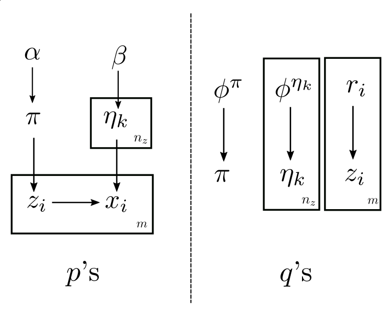
Given this structure we can write down the mean-field approximation:
\[\log q(z) = \mathbb E_{q(\eta)q(\pi)} (\log(x | z, \eta) + \log(z | \pi)) + C.\]
Both sides can be factored into per-sample expressions, giving us
\[\log q(z_i) = \mathbb E_{q(\eta)} \log p(x_i | z_i, \eta) + \mathbb E_{q(\pi)} \log p(z_i | \pi) + C\]
Therefore
\[\log r_{ik} = \log q(z_i = k) = \mathbb E_{q(\eta_k)} \log p(x_i | \eta_k) + \mathbb E_{q(\pi)} \log \pi_k + C. \qquad (9.1)\]
So the posterior of each \(z_i\) is categorical regardless of the $p$s and $q$s.
Computing the posterior of \(\pi\) and \(\eta\):
\[\log q(\pi) + \log q(\eta) = \log p(\pi) + \log p(\eta) + \sum_i \mathbb E_{q(z_i)} p(x_i | z_i, \eta) + \sum_i \mathbb E_{q(z_i)} p(z_i | \pi) + C.\]
So we can separate the terms involving \(\pi\) and those involving \(\eta\). First compute the posterior of \(\pi\):
\[\log q(\pi) = \log p(\pi) + \sum_i \mathbb E_{q(z_i)} \log p(z_i | \pi) = \log p(\pi) + \sum_i \sum_k r_{ik} \log \pi_k + C.\]
The right hand side is the log of a Dirichlet modulus the constant \(C\), from which we can update the posterior parameter \(\phi^\pi\):
\[\phi^\pi_k = \alpha + \sum_i r_{ik}. \qquad (9.3)\]
Similarly we can obtain the posterior of \(\eta\):
\[\log q(\eta) = \log p(\eta) + \sum_i \sum_k r_{ik} \log p(x_i | \eta_k) + C.\]
Again we can factor the terms with respect to \(k\) and get:
\[\log q(\eta_k) = \log p(\eta_k) + \sum_i r_{ik} \log p(x_i | \eta_k) + C. \qquad (9.5)\]
Here we can see why conjugate prior works. Mathematically, given a probability distribution \(p(x | \theta)\), the distribution \(p(\theta)\) is called conjugate prior of \(p(x | \theta)\) if \(\log p(\theta) + \log p(x | \theta)\) has the same form as \(\log p(\theta)\).
For example, the conjugate prior for the exponential family \(p(x | \theta) = h(x) \exp(\theta \cdot T(x) - A(\theta))\) where \(T\), \(A\) and \(h\) are some functions is \(p(\theta; \chi, \nu) \propto \exp(\chi \cdot \theta - \nu A(\theta))\).
Here what we want is a bit different from conjugate priors because of the coefficients \(r_{ik}\). But the computation carries over to the conjugate priors of the exponential family (try it yourself and you'll see). That is, if \(p(x_i | \eta_k)\) belongs to the exponential family
\[p(x_i | \eta_k) = h(x) \exp(\eta_k \cdot T(x) - A(\eta_k))\]
and if \(p(\eta_k)\) is the conjugate prior of \(p(x_i | \eta_k)\)
\[p(\eta_k) \propto \exp(\chi \cdot \eta_k - \nu A(\eta_k))\]
then \(q(\eta_k)\) has the same form as \(p(\eta_k)\), and from (9.5) we can compute the updates of \(\phi^{\eta_k}\):
\[\begin{aligned} \phi^{\eta_k}_1 &= \chi + \sum_i r_{ik} T(x_i), \qquad (9.7) \\ \phi^{\eta_k}_2 &= \nu + \sum_i r_{ik}. \qquad (9.9) \end{aligned}\]
So the mean field approximation for the fully Bayesian mixture model is the alternate iteration of (9.1) (E-step) and (9.3)(9.7)(9.9) (M-step) until convergence.
Fully Bayesian GMM
A typical example of fully Bayesian mixture models is the fully Bayesian Gaussian mixture model (Attias 2000, also called variational GMM in the literature). It is defined by applying the same modification to GMM as the difference between Fully Bayesian mixture model and the vanilla mixture model.
More specifically:
- \(p(z_{i}) = \text{Cat}(\pi)\) as in vanilla GMM
- \(p(\pi) = \text{Dir}(\alpha, \alpha, ..., \alpha)\) has Dirichlet distribution, the conjugate prior to the parameters of the categorical distribution.
- \(p(x_i | z_i = k) = p(x_i | \eta_k) = N(\mu_{k}, \Sigma_{k})\) as in vanilla GMM
- \(p(\mu_k, \Sigma_k) = \text{NIW} (\mu_0, \lambda, \Psi, \nu)\) is the normal-inverse-Wishart distribution, the conjugate prior to the mean and covariance matrix of the Gaussian distribution.
The E-step and M-step can be computed using (9.1) and (9.3)(9.7)(9.9) in the previous section. The details of the computation can be found in Chapter 10.2 of Bishop 2006 or Attias 2000.
LDA
As the second example of fully Bayesian mixture models, Latent Dirichlet allocation (LDA) (Blei-Ng-Jordan 2003) is the fully Bayesian version of pLSA2, with the following plate notations:
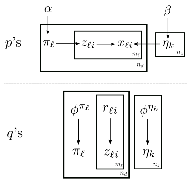
It is the smoothed version in the paper.
More specifically, on the basis of pLSA2, we add prior distributions to \(\eta\) and \(\pi\):
\[\begin{aligned} p(\eta_k) &= \text{Dir} (\beta, ..., \beta), \qquad k = 1 : n_z \\ p(\pi_\ell) &= \text{Dir} (\alpha, ..., \alpha), \qquad \ell = 1 : n_d \\ \end{aligned}\]
And as before, the prior of \(z\) is
\[p(z_{\ell, i}) = \text{Cat} (\pi_\ell), \qquad \ell = 1 : n_d, i = 1 : m\]
We also denote posterior distribution
\[\begin{aligned} q(\eta_k) &= \text{Dir} (\phi^{\eta_k}), \qquad k = 1 : n_z \\ q(\pi_\ell) &= \text{Dir} (\phi^{\pi_\ell}), \qquad \ell = 1 : n_d \\ p(z_{\ell, i}) &= \text{Cat} (r_{\ell, i}), \qquad \ell = 1 : n_d, i = 1 : m \end{aligned}\]
As before, in E-step we update \(r\), and in M-step we update \(\lambda\) and \(\gamma\).
But in the LDA paper, one treats optimisation over \(r\), \(\lambda\) and \(\gamma\) as a E-step, and treats \(\alpha\) and \(\beta\) as parameters, which is optmised over at M-step. This makes it more akin to the classical EM where the E-step is Bayesian and M-step MLE. This is more complicated, and we do not consider it this way here.
Plugging in (9.1) we obtain the updates at E-step
\[r_{\ell i k} \propto \exp(\psi(\phi^{\pi_\ell}_k) + \psi(\phi^{\eta_k}_{x_{\ell i}}) - \psi(\sum_w \phi^{\eta_k}_w)), \qquad (10)\]
where \(\psi\) is the digamma function. Similarly, plugging in (9.3)(9.7)(9.9), at M-step, we update the posterior of \(\pi\) and \(\eta\):
\[\begin{aligned} \phi^{\pi_\ell}_k &= \alpha + \sum_i r_{\ell i k}. \qquad (11)\\ %%}}$ %%As for $\eta$, we have %%{{$%align% %%\log q(\eta) &= \sum_k \log p(\eta_k) + \sum_{\ell, i} \mathbb E_{q(z_{\ell i})} \log p(x_{\ell i} | z_{\ell i}, \eta) \\ %%&= \sum_{k, j} (\sum_{\ell, i} r_{\ell i k} 1_{x_{\ell i} = j} + \beta - 1) \log \eta_{k j} %%}}$ %%which gives us %%{{$ \phi^{\eta_k}_w &= \beta + \sum_{\ell, i} r_{\ell i k} 1_{x_{\ell i} = w}. \qquad (12) \end{aligned}\]
So the algorithm iterates over (10) and (11)(12) until convergence.
DPMM
The Dirichlet process mixture model (DPMM) is like the fully Bayesian mixture model except \(n_z = \infty\), i.e. \(z\) can take any positive integer value.
The probability of \(z_i = k\) is defined using the so called stick-breaking process: let \(v_i \sim \text{Beta} (\alpha, \beta)\) be i.i.d. random variables with Beta distributions, then
\[\mathbb P(z_i = k | v_{1:\infty}) = (1 - v_1) (1 - v_2) ... (1 - v_{k - 1}) v_k.\]
So \(v\) plays a similar role to \(\pi\) in the previous models.
As before, we have that the distribution of \(x\) belongs to the exponential family:
\[p(x | z = k, \eta) = p(x | \eta_k) = h(x) \exp(\eta_k \cdot T(x) - A(\eta_k))\]
so the prior of \(\eta_k\) is
\[p(\eta_k) \propto \exp(\chi \cdot \eta_k - \nu A(\eta_k)).\]
Because of the infinities we can't directly apply the formulas in the general fully Bayesian mixture models. So let us carefully derive the whole thing again.
As before, we can write down the ELBO:
\[L(p(x, z, \theta), q(z, \theta)) = \mathbb E_{q(\theta)} \log {p(\theta) \over q(\theta)} + \mathbb E_{q(\theta) q(z)} \log {p(x, z | \theta) \over q(z)}.\]
Both terms are infinite series:
\[L(p, q) = \sum_{k = 1 : \infty} \mathbb E_{q(\theta_k)} \log {p(\theta_k) \over q(\theta_k)} + \sum_{i = 1 : m} \sum_{k = 1 : \infty} q(z_i = k) \mathbb E_{q(\theta)} \log {p(x_i, z_i = k | \theta) \over q(z_i = k)}.\]
There are several ways to deal with the infinities. One is to fix some level \(T > 0\) and set \(v_T = 1\) almost surely (Blei-Jordan 2006). This effectively turns the model into a finite one, and both terms become finite sums over \(k = 1 : T\).
Another walkaround (Kurihara-Welling-Vlassis 2007) is also a kind of truncation, but less heavy-handed: setting the posterior \(q(\theta) = q(\eta) q(v)\) to be:
\[q(\theta) = q(\theta_{1 : T}) p(\theta_{T + 1 : \infty}) =: q(\theta_{\le T}) p(\theta_{> T}).\]
That is, tie the posterior after \(T\) to the prior. This effectively turns the first term in the ELBO to a finite sum over \(k = 1 : T\), while keeping the second sum an infinite series:
\[L(p, q) = \sum_{k = 1 : T} \mathbb E_{q(\theta_k)} \log {p(\theta_k) \over q(\theta_k)} + \sum_i \sum_{k = 1 : \infty} q(z_i = k) \mathbb E_{q(\theta)} \log {p(x_i, z_i = k | \theta) \over q(z_i = k)}. \qquad (13)\]
The plate notation of this model is:
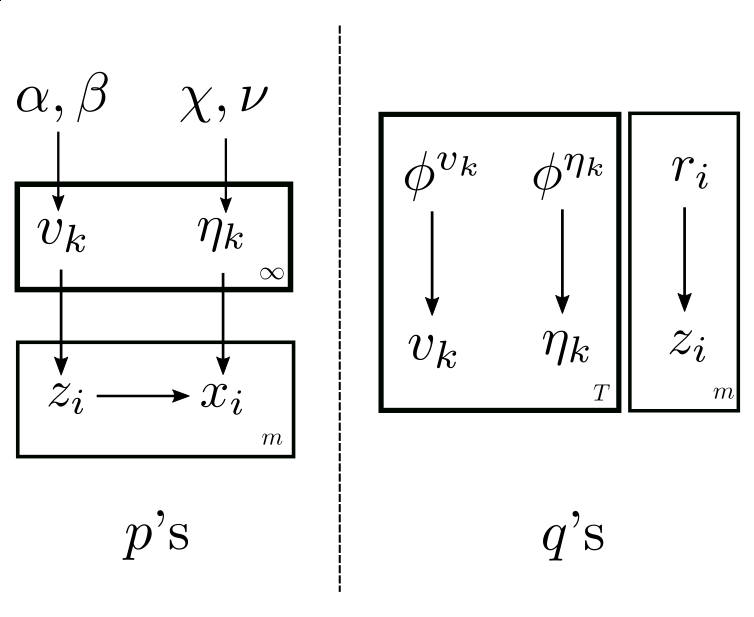
As it turns out, the infinities can be tamed in this case.
As before, the optimal \(q(z_i)\) is computed as
\[r_{ik} = q(z_i = k) = s_{ik} / S_i\]
where
\[\begin{aligned} s_{ik} &= \exp(\mathbb E_{q(\theta)} \log p(x_i, z_i = k | \theta)) \\ S_i &= \sum_{k = 1 : \infty} s_{ik}. \end{aligned}\]
Plugging this back to (13) we have
\[\begin{aligned} \sum_{k = 1 : \infty} r_{ik} &\mathbb E_{q(\theta)} \log {p(x_i, z_i = k | \theta) \over r_{ik}} \\ &= \sum_{k = 1 : \infty} r_{ik} \mathbb E_{q(\theta)} (\log p(x_i, z_i = k | \theta) - \mathbb E_{q(\theta)} \log p(x_i, z_i = k | \theta) + \log S_i) = \log S_i. \end{aligned}\]
So it all rests upon \(S_i\) being finite.
For \(k \le T + 1\), we compute the quantity \(s_{ik}\) directly. For \(k > T\), it is not hard to show that
\[s_{ik} = s_{i, T + 1} \exp((k - T - 1) \mathbb E_{p(w)} \log (1 - w)),\]
where \(w\) is a random variable with same distribution as \(p(v_k)\), i.e. \(\text{Beta}(\alpha, \beta)\).
Hence
\[S_i = \sum_{k = 1 : T} s_{ik} + {s_{i, T + 1} \over 1 - \exp(\psi(\beta) - \psi(\alpha + \beta))}\]
is indeed finite. Similarly we also obtain
\[q(z_i > k) = S^{-1} \left(\sum_{\ell = k + 1 : T} s_\ell + {s_{i, T + 1} \over 1 - \exp(\psi(\beta) - \psi(\alpha + \beta))}\right), k \le T \qquad (14)\]
Now let us compute the posterior of \(\theta_{\le T}\). In the following we exchange the integrals without justifying them (c.f. Fubini's Theorem). Equation (13) can be rewritten as
\[L(p, q) = \mathbb E_{q(\theta_{\le T})} \left(\log p(\theta_{\le T}) + \sum_i \mathbb E_{q(z_i) p(\theta_{> T})} \log {p(x_i, z_i | \theta) \over q(z_i)} - \log q(\theta_{\le T})\right).\]
Note that unlike the derivation of the mean-field approximation, we keep the \(- \mathbb E_{q(z)} \log q(z)\) term even though we are only interested in \(\theta\) at this stage. This is again due to the problem of infinities: as in the computation of \(S\), we would like to cancel out some undesirable unbounded terms using \(q(z)\). We now have
\[\log q(\theta_{\le T}) = \log p(\theta_{\le T}) + \sum_i \mathbb E_{q(z_i) p(\theta_{> T})} \log {p(x_i, z_i | \theta) \over q(z_i)} + C.\]
By plugging in \(q(z = k)\) we obtain
\[\log q(\theta_{\le T}) = \log p(\theta_{\le T}) + \sum_{k = 1 : \infty} q(z_i = k) \left(\mathbb E_{p(\theta_{> T})} \log {p(x_i, z_i = k | \theta) \over q(z_i = k)} - \mathbb E_{q(\theta)} \log {p(x_i, z_i = k | \theta) \over q(z_i = k)}\right) + C.\]
Again, we separate the \(v_k\)'s and the \(\eta_k\)'s to obtain
\[q(v_{\le T}) = \log p(v_{\le T}) + \sum_i \sum_k q(z_i = k) \left(\mathbb E_{p(v_{> T})} \log p(z_i = k | v) - \mathbb E_{q(v)} \log p (z_i = k | v)\right).\]
Denote by \(D_k\) the difference between the two expetations on the right hand side. It is easy to show that
\[D_k = \begin{cases} \log(1 - v_1) ... (1 - v_{k - 1}) v_k - \mathbb E_{q(v)} \log (1 - v_1) ... (1 - v_{k - 1}) v_k & k \le T\\ \log(1 - v_1) ... (1 - v_T) - \mathbb E_{q(v)} \log (1 - v_1) ... (1 - v_T) & k > T \end{cases}\]
so \(D_k\) is bounded. With this we can derive the update for \(\phi^{v, 1}\) and \(\phi^{v, 2}\):
\[\begin{aligned} \phi^{v, 1}_k &= \alpha + \sum_i q(z_i = k) \\ \phi^{v, 2}_k &= \beta + \sum_i q(z_i > k), \end{aligned}\]
where \(q(z_i > k)\) can be computed as in (14).
When it comes to \(\eta\), we have
\[\log q(\eta_{\le T}) = \log p(\eta_{\le T}) + \sum_i \sum_{k = 1 : \infty} q(z_i = k) (\mathbb E_{p(\eta_k)} \log p(x_i | \eta_k) - \mathbb E_{q(\eta_k)} \log p(x_i | \eta_k)).\]
Since \(q(\eta_k) = p(\eta_k)\) for \(k > T\), the inner sum on the right hand side is a finite sum over \(k = 1 : T\). By factorising \(q(\eta_{\le T})\) and \(p(\eta_{\le T})\), we have
\[\log q(\eta_k) = \log p(\eta_k) + \sum_i q(z_i = k) \log (x_i | \eta_k) + C,\]
which gives us
\[\begin{aligned} \phi^{\eta, 1}_k &= \xi + \sum_i q(z_i = k) T(x_i) \\ \phi^{\eta, 2}_k &= \nu + \sum_i q(z_i = k). \end{aligned}\]
SVI
In variational inference, the computation of some parameters are more expensive than others.
For example, the computation of M-step is often much more expensive than that of E-step:
- In the vanilla mixture models with the EM algorithm, the update of \(\theta\) requires the computation of \(r_{ik}\) for all \(i = 1 : m\), see Eq (2.3).
- In the fully Bayesian mixture model with mean field approximation, the updates of \(\phi^\pi\) and \(\phi^\eta\) require the computation of a sum over all samples (see Eq (9.3)(9.7)(9.9)).
Similarly, in pLSA2 (resp. LDA), the updates of \(\eta_k\) (resp. \(\phi^{\eta_k}\)) requires a sum over \(\ell = 1 : n_d\), whereas the updates of other parameters do not.
In these cases, the parameter that requires more computations are called global and the other ones local.
Stochastic variational inference (SVI, Hoffman-Blei-Wang-Paisley 2012) addresses this problem in the same way as stochastic gradient descent improves efficiency of gradient descent.
Each time SVI picks a sample, updates the corresponding local parameters, and computes the update of the global parameters as if all the \(m\) samples are identical to the picked sample. Finally it incorporates this global parameter value into previous computations of the global parameters, by means of an exponential moving average.
As an example, here's SVI applied to LDA:
- Set \(t = 1\).
- Pick \(\ell\) uniformly from \(\{1, 2, ..., n_d\}\).
- Repeat until convergence:
- Compute \((r_{\ell i k})_{i = 1 : m, k = 1 : n_z}\) using (10).
- Compute \((\phi^{\pi_\ell}_k)_{k = 1 : n_z}\) using (11).
- Compute \((\tilde \phi^{\eta_k}_w)_{k = 1 : n_z, w = 1 : n_x}\) using the following formula (compare with (12)) \[\tilde \phi^{\eta_k}_w = \beta + n_d \sum_{i} r_{\ell i k} 1_{x_{\ell i} = w}\]
- Update the exponential moving average \((\phi^{\eta_k}_w)_{k = 1 : n_z, w = 1 : n_x}\): \[\phi^{\eta_k}_w = (1 - \rho_t) \phi^{\eta_k}_w + \rho_t \tilde \phi^{\eta_k}_w\]
- Increment \(t\) and go back to Step 2.
In the original paper, \(\rho_t\) needs to satisfy some conditions that guarantees convergence of the global parameters:
\[\begin{aligned} \sum_t \rho_t = \infty \\ \sum_t \rho_t^2 < \infty \end{aligned}\]
and the choice made there is
\[\rho_t = (t + \tau)^{-\kappa}\]
for some \(\kappa \in (.5, 1]\) and \(\tau \ge 0\).
AEVB
SVI adds to variational inference stochastic updates similar to stochastic gradient descent. Why not just use neural networks with stochastic gradient descent while we are at it? Autoencoding variational Bayes (AEVB) (Kingma-Welling 2013) is such an algorithm.
Let's look back to the original problem of maximising the ELBO:
\[\max_{\theta, q} \sum_{i = 1 : m} L(p(x_i | z_i; \theta) p(z_i; \theta), q(z_i))\]
Since for any given \(\theta\), the optimal \(q(z_i)\) is the posterior \(p(z_i | x_i; \theta)\), the problem reduces to
\[\max_{\theta} \sum_i L(p(x_i | z_i; \theta) p(z_i; \theta), p(z_i | x_i; \theta))\]
Let us assume \(p(z_i; \theta) = p(z_i)\) is independent of \(\theta\) to simplify the problem. In the old mixture models, we have \(p(x_i | z_i; \theta) = p(x_i; \eta_{z_i})\), which we can generalise to \(p(x_i; f(\theta, z_i))\) for some function \(f\). Using Beyes' theorem we can also write down \(p(z_i | x_i; \theta) = q(z_i; g(\theta, x_i))\) for some function \(g\). So the problem becomes
\[\max_{\theta} \sum_i L(p(x_i; f(\theta, z_i)) p(z_i), q(z_i; g(\theta, x_i)))\]
In some cases \(g\) can be hard to write down or compute. AEVB addresses this problem by replacing \(g(\theta, x_i)\) with a neural network \(g_\phi(x_i)\) with input \(x_i\) and some separate parameters \(\phi\). It also replaces \(f(\theta, z_i)\) with a neural network \(f_\theta(z_i)\) with input \(z_i\) and parameters \(\theta\). And now the problem becomes
\[\max_{\theta, \phi} \sum_i L(p(x_i; f_\theta(z_i)) p(z_i), q(z_i; g_\phi(x_i))).\]
The objective function can be written as
\[\sum_i \mathbb E_{q(z_i; g_\phi(x_i))} \log p(x_i; f_\theta(z_i)) - D(q(z_i; g_\phi(x_i)) || p(z_i)).\]
The first term is called the negative reconstruction error, like the \(- \|decoder(encoder(x)) - x\|\) in autoencoders, which is where the "autoencoder" in the name comes from.
The second term is a regularisation term that penalises the posterior \(q(z_i)\) that is very different from the prior \(p(z_i)\). We assume this term can be computed analytically.
So only the first term requires computing.
We can approximate the sum over \(i\) in a similar fashion as SVI: pick \(j\) uniformly randomly from \(\{1 ... m\}\) and treat the whole dataset as \(m\) replicates of \(x_j\), and approximate the expectation using Monte-Carlo:
\[U(x_i, \theta, \phi) := \sum_i \mathbb E_{q(z_i; g_\phi(x_i))} \log p(x_i; f_\theta(z_i)) \approx m \mathbb E_{q(z_j; g_\phi(x_j))} \log p(x_j; f_\theta(z_j)) \approx {m \over L} \sum_{\ell = 1}^L \log p(x_j; f_\theta(z_{j, \ell})),\]
where each \(z_{j, \ell}\) is sampled from \(q(z_j; g_\phi(x_j))\).
But then it is not easy to approximate the gradient over \(\phi\). One can use the log trick as in policy gradients, but it has the problem of high variance. In policy gradients this is overcome by using baseline subtractions. In the AEVB paper it is tackled with the reparameterisation trick.
Assume there exists a transformation \(T_\phi\) and a random variable \(\epsilon\) with distribution independent of \(\phi\) or \(\theta\), such that \(T_\phi(x_i, \epsilon)\) has distribution \(q(z_i; g_\phi(x_i))\). In this case we can rewrite \(U(x, \phi, \theta)\) as
\[\sum_i \mathbb E_{\epsilon \sim p(\epsilon)} \log p(x_i; f_\theta(T_\phi(x_i, \epsilon))),\]
This way one can use Monte-Carlo to approximate \(\nabla_\phi U(x, \phi, \theta)\):
\[\nabla_\phi U(x, \phi, \theta) \approx {m \over L} \sum_{\ell = 1 : L} \nabla_\phi \log p(x_j; f_\theta(T_\phi(x_j, \epsilon_\ell))),\]
where each \(\epsilon_{\ell}\) is sampled from \(p(\epsilon)\). The approximation of \(U(x, \phi, \theta)\) itself can be done similarly.
VAE
As an example of AEVB, the paper introduces variational autoencoder (VAE), with the following instantiations:
- The prior \(p(z_i) = N(0, I)\) is standard normal, thus independent of \(\theta\).
- The distribution \(p(x_i; \eta)\) is either Gaussian or categorical.
- The distribution \(q(z_i; \mu, \Sigma)\) is Gaussian with diagonal covariance matrix. So \(g_\phi(z_i) = (\mu_\phi(x_i), \text{diag}(\sigma^2_\phi(x_i)_{1 : d}))\). Thus in the reparameterisation trick \(\epsilon \sim N(0, I)\) and \(T_\phi(x_i, \epsilon) = \epsilon \odot \sigma_\phi(x_i) + \mu_\phi(x_i)\), where \(\odot\) is elementwise multiplication.
- The KL divergence can be easily computed analytically as \(- D(q(z_i; g_\phi(x_i)) || p(z_i)) = {d \over 2} + \sum_{j = 1 : d} \log\sigma_\phi(x_i)_j - {1 \over 2} \sum_{j = 1 : d} (\mu_\phi(x_i)_j^2 + \sigma_\phi(x_i)_j^2)\).
With this, one can use backprop to maximise the ELBO.
Fully Bayesian AEVB
Let us turn to fully Bayesian version of AEVB. Again, we first recall the ELBO of the fully Bayesian mixture models:
\[L(p(x, z, \pi, \eta; \alpha, \beta), q(z, \pi, \eta; r, \phi)) = L(p(x | z, \eta) p(z | \pi) p(\pi; \alpha) p(\eta; \beta), q(z; r) q(\eta; \phi^\eta) q(\pi; \phi^\pi)).\]
We write \(\theta = (\pi, \eta)\), rewrite \(\alpha := (\alpha, \beta)\), \(\phi := r\), and \(\gamma := (\phi^\eta, \phi^\pi)\). Furthermore, as in the half-Bayesian version we assume \(p(z | \theta) = p(z)\), i.e. \(z\) does not depend on \(\theta\). Similarly we also assume \(p(\theta; \alpha) = p(\theta)\). Now we have
\[L(p(x, z, \theta; \alpha), q(z, \theta; \phi, \gamma)) = L(p(x | z, \theta) p(z) p(\theta), q(z; \phi) q(\theta; \gamma)).\]
And the objective is to maximise it over \(\phi\) and \(\gamma\). We no longer maximise over \(\theta\), because it is now a random variable, like \(z\). Now let us transform it to a neural network model, as in the half-Bayesian case:
\[L\left(\left(\prod_{i = 1 : m} p(x_i; f_\theta(z_i))\right) \left(\prod_{i = 1 : m} p(z_i) \right) p(\theta), \left(\prod_{i = 1 : m} q(z_i; g_\phi(x_i))\right) q(\theta; h_\gamma(x))\right).\]
where \(f_\theta\), \(g_\phi\) and \(h_\gamma\) are neural networks. Again, by separating out KL-divergence terms, the above formula becomes
\[\sum_i \mathbb E_{q(\theta; h_\gamma(x))q(z_i; g_\phi(x_i))} \log p(x_i; f_\theta(z_i)) - \sum_i D(q(z_i; g_\phi(x_i)) || p(z_i)) - D(q(\theta; h_\gamma(x)) || p(\theta)).\]
Again, we assume the latter two terms can be computed analytically. Using reparameterisation trick, we write
\[\begin{aligned} \theta &= R_\gamma(\zeta, x) \\ z_i &= T_\phi(\epsilon, x_i) \end{aligned}\]
for some transformations \(R_\gamma\) and \(T_\phi\) and random variables \(\zeta\) and \(\epsilon\) so that the output has the desired distributions.
Then the first term can be written as
\[\mathbb E_{\zeta, \epsilon} \log p(x_i; f_{R_\gamma(\zeta, x)} (T_\phi(\epsilon, x_i))),\]
so that the gradients can be computed accordingly.
Again, one may use Monte-Carlo to approximate this expetation.
References
- Attias, Hagai. "A variational baysian framework for graphical models." In Advances in neural information processing systems, pp. 209-215. 2000.
- Bishop, Christopher M. Neural networks for pattern recognition. Springer. 2006.
- Blei, David M., and Michael I. Jordan. "Variational Inference for Dirichlet Process Mixtures." Bayesian Analysis 1, no. 1 (March 2006): 121–43. https://doi.org/10.1214/06-BA104.
- Blei, David M., Andrew Y. Ng, and Michael I. Jordan. "Latent Dirichlet Allocation." Journal of Machine Learning Research 3, no. Jan (2003): 993–1022.
- Hofmann, Thomas. "Latent Semantic Models for Collaborative Filtering." ACM Transactions on Information Systems 22, no. 1 (January 1, 2004): 89–115. https://doi.org/10.1145/963770.963774.
- Hofmann, Thomas. "Learning the similarity of documents: An information-geometric approach to document retrieval and categorization." In Advances in neural information processing systems, pp. 914-920. 2000.
- Hoffman, Matt, David M. Blei, Chong Wang, and John Paisley. "Stochastic Variational Inference." ArXiv:1206.7051 [Cs, Stat], June 29, 2012. http://arxiv.org/abs/1206.7051.
- Kingma, Diederik P., and Max Welling. "Auto-Encoding Variational Bayes." ArXiv:1312.6114 [Cs, Stat], December 20, 2013. http://arxiv.org/abs/1312.6114.
- Kurihara, Kenichi, Max Welling, and Nikos Vlassis. "Accelerated variational Dirichlet process mixtures." In Advances in neural information processing systems, pp. 761-768. 2007.
- Sudderth, Erik Blaine. "Graphical models for visual object recognition and tracking." PhD diss., Massachusetts Institute of Technology, 2006.